Comparison to CCL
This notebook compares the implementation from jax_cosmo to CCL
[1]:
%pylab inline
import os
os.environ['JAX_ENABLE_X64']='True'

import pyccl as ccl
import jax
from jax_cosmo import Cosmology, background
Populating the interactive namespace from numpy and matplotlib
[2]:
# We first define equivalent CCL and jax_cosmo cosmologies
cosmo_ccl = ccl.Cosmology(
    Omega_c=0.3, Omega_b=0.05, h=0.7, sigma8 = 0.8, n_s=0.96, Neff=0,
    transfer_function='eisenstein_hu', matter_power_spectrum='halofit')

cosmo_jax = Cosmology(Omega_c=0.3, Omega_b=0.05, h=0.7, sigma8 = 0.8, n_s=0.96,
                      Omega_k=0., w0=-1., wa=0.)
Comparing background cosmology
[3]:
# Test array of scale factors
a = np.linspace(0.01, 1.)
[4]:
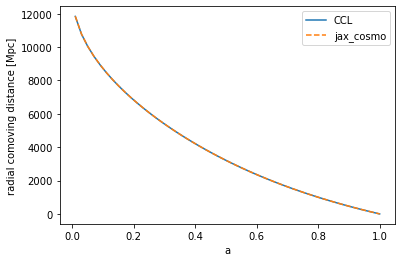
# Testing the radial comoving distance
chi_ccl = ccl.comoving_radial_distance(cosmo_ccl, a)
chi_jax = background.radial_comoving_distance(cosmo_jax, a)/cosmo_jax.h

plot(a, chi_ccl, label='CCL')
plot(a, chi_jax, '--', label='jax_cosmo')
legend()
xlabel('a')
ylabel('radial comoving distance [Mpc]')
/home/francois/.local/lib/python3.8/site-packages/jax/lib/xla_bridge.py:116: UserWarning: No GPU/TPU found, falling back to CPU.
  warnings.warn('No GPU/TPU found, falling back to CPU.')
[4]:
Text(0, 0.5, 'radial comoving distance [Mpc]')
[5]:
# Testing the angular comoving distance
chi_ccl = ccl.comoving_angular_distance(cosmo_ccl, a)
chi_jax = background.transverse_comoving_distance(cosmo_jax, a)/cosmo_jax.h

plot(a, chi_ccl, label='CCL')
plot(a, chi_jax, '--', label='jax_cosmo')
legend()
xlabel('a')
ylabel('angular comoving distance [Mpc]')
[5]:
Text(0, 0.5, 'angular comoving distance [Mpc]')

[6]:
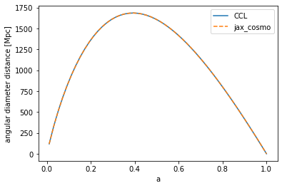
# Testing the angular diameter distance
chi_ccl = ccl.angular_diameter_distance(cosmo_ccl, a)
chi_jax = background.angular_diameter_distance(cosmo_jax, a)/cosmo_jax.h

plot(a, chi_ccl, label='CCL')
plot(a, chi_jax, '--', label='jax_cosmo')
legend()
xlabel('a')
ylabel('angular diameter distance [Mpc]')
[6]:
Text(0, 0.5, 'angular diameter distance [Mpc]')
[7]:
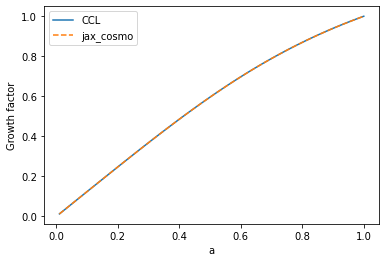
# Comparing the growth factor
plot(a, ccl.growth_factor(cosmo_ccl,a), label='CCL')
plot(a, background.growth_factor(cosmo_jax, a), '--', label='jax_cosmo')
legend()
xlabel('a')
ylabel('Growth factor')
[7]:
Text(0, 0.5, 'Growth factor')
[8]:
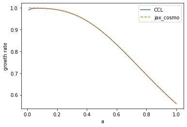
# Comparing linear growth rate
plot(a, ccl.growth_rate(cosmo_ccl,a), label='CCL')
plot(a, background.growth_rate(cosmo_jax, a), '--', label='jax_cosmo')
legend()
xlabel('a')
ylabel('growth rate')
[8]:
Text(0, 0.5, 'growth rate')
Comparing matter power spectrum
[9]:
from jax_cosmo.power import linear_matter_power, nonlinear_matter_power
[9]:
k = np.logspace(-3,-0.5)
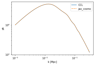
[10]:
#Let's have a look at the linear power
pk_ccl = ccl.linear_matter_power(cosmo_ccl, k, 1.0)
pk_jax = linear_matter_power(cosmo_jax, k/cosmo_jax.h, a=1.0)

loglog(k,pk_ccl,label='CCL')
loglog(k,pk_jax/cosmo_jax.h**3, '--', label='jax_cosmo')
legend()
xlabel('k [Mpc]')
ylabel('pk');
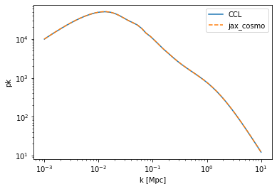
[11]:
k = np.logspace(-3,1)
#Let's have a look at the non linear power
pk_ccl = ccl.nonlin_matter_power(cosmo_ccl, k, 1.0)
pk_jax = nonlinear_matter_power(cosmo_jax, k/cosmo_jax.h, a=1.0)

loglog(k,pk_ccl,label='CCL')
loglog(k,pk_jax/cosmo_jax.h**3, '--', label='jax_cosmo')
legend()
xlabel('k [Mpc]')
ylabel('pk');
Comparing angular cl
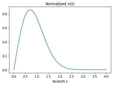
[12]:
from jax_cosmo.redshift import smail_nz

# Let's define a redshift distribution
# with a Smail distribution with a=1, b=2, z0=1
nz = smail_nz(1.,2., 1.)
[13]:
z = linspace(0,4,1024)
plot(z, nz(z))
xlabel(r'Redshift $z$');
title('Normalized n(z)');
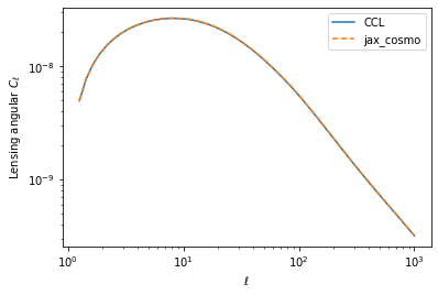
[14]:
from jax_cosmo.angular_cl import angular_cl
from jax_cosmo import probes

# Let's first compute some Weak Lensing cls
tracer_ccl = ccl.WeakLensingTracer(cosmo_ccl, (z, nz(z)), use_A_ia=False)
tracer_jax = probes.WeakLensing([nz])

ell = np.logspace(0.1,3)

cl_ccl = ccl.angular_cl(cosmo_ccl, tracer_ccl, tracer_ccl, ell)
cl_jax = angular_cl(cosmo_jax, ell, [tracer_jax])
[15]:
loglog(ell, cl_ccl,label='CCL')
loglog(ell, cl_jax[0], '--', label='jax_cosmo')

legend()
xlabel(r'$\ell$')
ylabel(r'Lensing angular $C_\ell$')
[15]:
Text(0, 0.5, 'Lensing angular $C_\\ell$')
[16]:
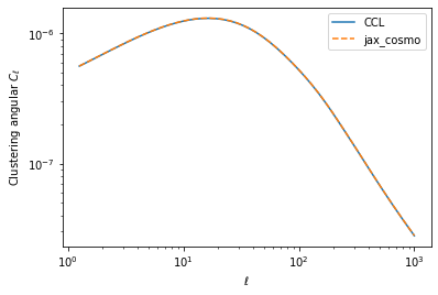
# Let's try galaxy clustering now
from jax_cosmo.bias import constant_linear_bias

# We define a trivial bias model
bias = constant_linear_bias(1.)

tracer_ccl_n = ccl.NumberCountsTracer(cosmo_ccl,
                                      has_rsd=False,
                                      dndz=(z, nz(z)),
                                      bias=(z, bias(cosmo_jax, z)))
tracer_jax_n = probes.NumberCounts([nz], bias)

cl_ccl = ccl.angular_cl(cosmo_ccl, tracer_ccl_n, tracer_ccl_n, ell)
cl_jax = angular_cl(cosmo_jax, ell, [tracer_jax_n])
[17]:
import jax_cosmo.constants as cst
loglog(ell, cl_ccl,label='CCL')
loglog(ell, cl_jax[0], '--', label='jax_cosmo')

legend()
xlabel(r'$\ell$')
ylabel(r'Clustering angular $C_\ell$')
[17]:
Text(0, 0.5, 'Clustering angular $C_\\ell$')
[18]:
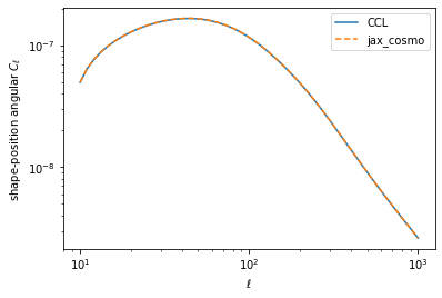
# And  finally.... a cross-spectrum

cl_ccl = ccl.angular_cl(cosmo_ccl, tracer_ccl, tracer_ccl_n, ell)
cl_jax = angular_cl(cosmo_jax, ell, [tracer_jax, tracer_jax_n])
[19]:
ell = np.logspace(1,3)

loglog(ell, cl_ccl,label='CCL')
loglog(ell, cl_jax[1], '--', label='jax_cosmo')

legend()
xlabel(r'$\ell$')
ylabel(r'shape-position angular $C_\ell$')
[19]:
Text(0, 0.5, 'shape-position angular $C_\\ell$')
[ ]: